Mixed Effects Models in R
Phillip M Alday
17. July 2013

This work is licensed under a Creative Commons Attribution-NonCommercial-ShareAlike 3.0 Unported License
Today's data: Sleep Study
Reaction: RT in msDays: day 0 is normal sleep baseline (interval da -> Numeric)Subject: numbered (categorical, non ordinal -> Factor)
In R
> # example data providedy by lme4
> library(lme4)
> data(sleepstudy)
> # for more info, try ?sleepstudy
> library(lattice)  # provides some nice plotting functions
> str(sleepstudy)## 'data.frame': 180 obs. of 3 variables:
## $ Reaction: num 250 259 251 321 357 ...
## $ Days : num 0 1 2 3 4 5 6 7 8 9 ...
## $ Subject : Factor w/ 18 levels "308","309","310",..: 1 1 1 1 1 1 1 1 1 1 ...A quick warning
- timeo danaos et dona ferentes!
- Relax, it'll be okay.
Back to basics
Linear Regression
> # simple scatter plot
> sleep.xy <- xyplot(Reaction~Days,data=sleepstudy,
+                    xlab = "Days of sleep deprivation",
+                    ylab = "Average reaction time (ms)")
> sleep.xy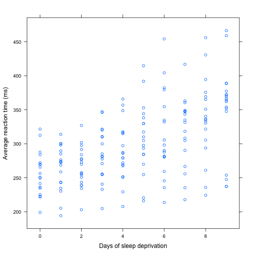
Make a linear model
- basic line, no error term: y = mx + b
- dep = slope*indep + baseline.offset
- outcome = (model) + error
Fit a line
- Fit a line to observed data with magic and matrices:
- Y = β1X + β0 + ε
- Y = β2X + β1X + β0 + ε
- Y = β3X + β2X + β1X + β0 + ε
- ...
R has this built in:
> sleep.lm <- lm(Reaction ~ Days, data = sleepstudy)additional predictors with
+(no interaction) or*(interaction)
Add a regression line with lattice graphics
> # update() effectively performs the previous call for us PLUS other
> # options we add now
> sleep.xy <- update(sleep.xy, type = c("p", "r"))  # p for points, r for regression
> sleep.xy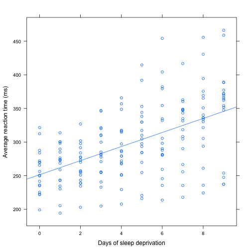
Model summary
> summary(sleep.lm)##
## Call:
## lm(formula = Reaction ~ Days, data = sleepstudy)
##
## Residuals:
## Min 1Q Median 3Q Max
## -110.85 -27.48 1.55 26.14 139.95
##
## Coefficients:
## Estimate Std. Error t value Pr(>|t|)
## (Intercept) 251.41 6.61 38.03 < 2e-16 ***
## Days 10.47 1.24 8.45 9.9e-15 ***
## ---
## Signif. codes: 0 '***' 0.001 '**' 0.01 '*' 0.05 '.' 0.1 ' ' 1
##
## Residual standard error: 47.7 on 178 degrees of freedom
## Multiple R-squared: 0.286, Adjusted R-squared: 0.282
## F-statistic: 71.5 on 1 and 178 DF, p-value: 9.89e-15Not a great fit!
Residuals for all data
> # convenient lattice function for residuals
> rfs(sleep.lm)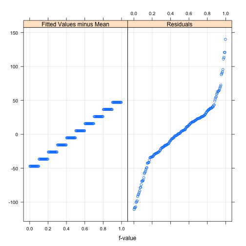
Residuals for a single subject
> sleep.lm.vp1 <- lm(Reaction ~ Days,
+                    data=sleepstudy[sleepstudy$Subject=="308",])
> rfs(sleep.lm.vp1)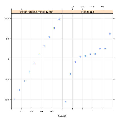
Models for single subjects
> sleep.xy.bysubj <- xyplot(Reaction ~ Days|Subject,
+                           data=sleepstudy,
+                           xlab = "Days of sleep deprivation",
+                           ylab = "Average reaction time (ms)")
> sleep.xy.bysubj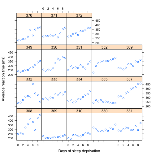
With regression lines
> sleep.xy.bysubj <- update(sleep.xy.bysubj, type = c("p", "r"))
> sleep.xy.bysubj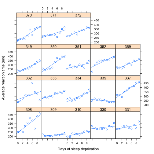
Variance and Repeated Measures
- Inter- and Intra- variance
- random jitter from our choice of sample population
- each subject fulfills a certain "condition", but random error pro instance of the condition
- similar idea for item analysis in linguistic designs
Fixed vs Random Effects
- Model subjects as fixed effect?
- only when we want to make intrasample predictions
- i.e. sample==population
- fixed means known variance / manipulation
- fixed-effects: directed, preferably "exhaustive" manipulation
- Model subjects as random effects?
- "random" means unknown variance
- error term is a random effect
- correction for the error resulting from our particular choice of sample
- correction per grouping for slope and intercept possible
- error term per grouping!
Mixed Effects Models
- "Mixed" because both fixed random effects are used
- Same basic formula syntax
dep ~ indep | group additional
(indep|group)terms for random effects> sleep.lmer <- lmer(Reaction ~ Days + (1|Subject), + data=sleepstudy)
> ?formulaModel Summary
> summary(sleep.lmer)## Linear mixed model fit by REML
## Formula: Reaction ~ Days + (1 | Subject)
## Data: sleepstudy
## AIC BIC logLik deviance REMLdev
## 1794 1807 -893 1794 1786
## Random effects:
## Groups Name Variance Std.Dev.
## Subject (Intercept) 1378 37.1
## Residual 960 31.0
## Number of obs: 180, groups: Subject, 18
##
## Fixed effects:
## Estimate Std. Error t value
## (Intercept) 251.405 9.746 25.8
## Days 10.467 0.804 13.0
##
## Correlation of Fixed Effects:
## (Intr)
## Days -0.371Fixed effect structure
- Package
ezezMixed()as a convenience for exploring fixed effectsezPredict()useful for plotting regression lines
- Package
effects - Package
lmerTest - Package
languageR - Package
LMERConvenienceFunctions - Package
lmtest - (example and special purpose code from Phillip)
Random effect structure
- combine by-subject and by-item analyses in one step
- cf. Clark (1973)
Random effect structure
- Early idea: build up from minimal structure until improvements don't bring you anything on ANOVA (Baayen et al. 2008 )
- New idea: Use the most complicated random effects structure possible (Barr et al. 2013 )
Random effect structure
- Possible random effect structures for ONE fixed factor:
- Intercepts only by random factor:
(1 | random.factor) - Slopes only by random factor:
(0 + fixed.factor | random.factor) - Intercepts and slopes by random factor:
(1 + fixed.factor | random.factor) - Intercept and slope, separately, by random factor:
(1 | random.factor) + (0 + fixed.factor | random.factor)
- Intercepts only by random factor:
Models
> # REML is a "shortcut" that invalidates anova()
> sleep.lmer <- update(sleep.lmer,REML=FALSE)
> # same as (Days|Subject)
> sleep.lmer.slopes <- lmer(Reaction ~ Days + (1+Days|Subject),
+                            data=sleepstudy,REML=FALSE)
> sleep.lmer.slopes.int <- lmer(Reaction ~ Days + (1|Subject) +
+                                (0+Days|Subject),
+                                data=sleepstudy,REML=FALSE)
Comparing Models
> # can only be used for nested models!
> anova(sleep.lmer, sleep.lmer.slopes, sleep.lmer.slopes.int)
## Data: sleepstudy
## Models:
## sleep.lmer: Reaction ~ Days + (1 | Subject)
## sleep.lmer.slopes.int: Reaction ~ Days + (1 | Subject) + (0 + Days | Subject)
## sleep.lmer.slopes: Reaction ~ Days + (1 + Days | Subject)
## Df AIC BIC logLik Chisq Chi Df Pr(>Chisq)
## sleep.lmer 4 1802 1815 -897
## sleep.lmer.slopes.int 5 1762 1778 -876 42.08 1 8.8e-11 ***
## sleep.lmer.slopes 6 1764 1783 -876 0.06 1 0.8
## ---
## Signif. codes: 0 '***' 0.001 '**' 0.01 '*' 0.05 '.' 0.1 ' ' 1Judging Fit
Relationship to ANOVA
ezANOVA()depends onaov()which depends onlm()anova()can be used to compare existinglm()s- linear models compared with F and t tests
- no continuous predictors with ANOVA
- ANOVA works on per-subject item averages and examines variance over subjects for each condition
- MEMs work at an individual trial level and can accomodate empty cells and unbalanced designs!
ezANOVA()
> # hide startup output
> suppressPackageStartupMessages(library(ez))
> sleep.ez <- ezANOVA(sleepstudy,
+                     dv=.(Reaction),
+                     wid=.(Subject),
+                     within=.(Days),
+                     detailed=TRUE,
+             # we'll take a look at the aov() in a sec
+                     return_aov=TRUE)
## Warning: "Days" will be treated as numeric.## Warning: There is at least one numeric within variable, therefore aov()
## will be used for computation and no assumption checks will be obtained.> sleep.ez$ANOVA## Effect DFn DFd SSn SSd F p p<.05 ges
## 1 Days 1 17 162703 60322 45.85 3.264e-06 * 0.7295
aov() from ezANOVA()
> sleep.ez$aov##
## Call:
## aov(formula = formula(aov_formula), data = data)
##
## Grand Mean: 298.5
##
## Stratum 1: Subject
##
## Terms:
## Residuals
## Sum of Squares 250618
## Deg. of Freedom 17
##
## Residual standard error: 121.4
##
## Stratum 2: Subject:Days
##
## Terms:
## Days Residuals
## Sum of Squares 162703 60322
## Deg. of Freedom 1 17
##
## Residual standard error: 59.57
## Estimated effects are balanced
##
## Stratum 3: Within
##
## Terms:
## Residuals
## Sum of Squares 94312
## Deg. of Freedom 144
##
## Residual standard error: 25.59
formula from aov() from ezANOVA()
> aov.formula <- formula(attr(sleep.ez$aov, "terms"))
> print(aov.formula, showEnv = FALSE)
## Reaction ~ Days + Error(Subject/(Days))Possible warning messages
- Convergence warnings: you don't have enough data for the proposed model structure
- Singular: perfect multicollinearity (at least one variable is linear combination of the others)
- Not positive definite: matrix not greater than "zero"; too much correlation / collinearity, not enough data
Extensions of linear models to non-linear data
- traditional linear models can be extended to model other types of data such as binary (e.g. yes/no responses)
- basically works by strapping a transformation (link function) onto the front and back ends -- R does this for you!
- fixed effects:
glm() - mixed effects:
glmer()
Family types
- binomial: (aka logistic regression)
binary ~ continuous - Gaussian: (normal linear regression)
continuous ~ continuousandcontinuous ~ categegorial - Gamma:
continuous ~ exp(continuous)(exponential response) - Poisson:
count ~ continuous - (inverse.gaussian, quasi, quasibinomial, quasipoisson)
Binomial models
- casuality of grouping
- traditional t-test vs. detection prediction
- Johannes' data
- existence / evidence for a priori categories
- connecting theory and empiry
- difficult vs non difficult violations
behavioral ~ eeg- performance (cf. VanRullen (2011)
- anomaly detection
- Sarah's data
Plain Text Rocks!
- View this presentation online at https://palday.bitbucket.org/presentations/mem.html
- Source code (R Markdown) available at https://bitbucket.org/palday/mixed-models
- Hats off to reveal.js and
knitr
(More) References
- Stack Exchange and Cross Validated
- GLM Families
- Especially relevant questions
- Florian Jaeger's blog
- Jonathan Harrington (phonetics prof. in Munich):
- Mixed Models (in German)
- Generalized Linear Mixed Models (in English)
- Tutorial for sociolinguists
- lmer, p-values and all that
- Understanding
glmer()output - Package
nlme(older, more specialized MEM implementation), see also here
- Tutorial from
lme4coauthor: (Bolker et al. 2009 ) - Modelling interindividual differences via mixed models
- In corpus linguistics / dialectology: Wieling et al. (2011)